Logistic Regression

 Logistic Regression

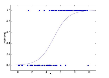
Don’t get confused by its name! It is a classification not a regression algorithm. It is used to estimate discrete values ( Binary values like 0/1, yes/no, true/false ) based on given set of independent variable(s). In simple words, it predicts the probability of occurrence of an event by fitting data to a logit function. Hence, it is also known as logistic regression. Since, it predicts the probability, its output values lies between 0 and 1 (as expected). 

Again, let us try and understand this through a simple example.

Let’s say your friend gives you a puzzle to solve. There are only 2 outcome scenarios – either you solve it or you don’t. Now imagine, that you are being given wide range of puzzles / quizzes in an attempt to understand which subjects you are good at. The outcome to this study would be something like this – if you are given a trigonometry based tenth grade problem, you are 70% likely to solve it. On the other hand, if it is grade fifth history question, the probability of getting an answer is only 30%. This is what Logistic Regression provides you.

Coming to the math, the log odds of the outcome is modeled as a linear combination of the predictor variables.

odds= p/ (1-p) = probability of event occurrence / probab ility of not event occurrence ln(odds) = ln(p/(1-p)) logit(p) = ln(p/(1-p)) = b0+b1X1+b2X2+b3X3....+bkXk

Above, p is the probability of presence of the characteristic of interest. It chooses parameters that maximize the likelihood of observing the sample values rather than that minimize the sum of squared errors (like in ordinary regression).

Now, you may ask, why take a log? For the sake of simplicity, let’s just say that this is one of the best mathematical way to replicate a step function. I can go in more details, but that will beat the purpose of this article.

 

Example in Python for Logistic Regresssion




import pandas as pd

import numpy as np

import seaborn as sns

import matplotlib.pyplot as plt

from sklearn.model_selection import train_test_split

from sklearn.linear_model import LogisticRegression

from sklearn.metrics import classification_report

from sklearn.metrics import confusion_matrix,accuracy_score

 

# load the dataset

df = pd.read_csv(r'C:UsersDocumentsdata.csv')

# defining feature matrix(X) and response vector(y)

x = df.drop('Home', axis=1)

y = df['Home']




# splitting X and y into training and testing sets

x_train, x_test, y_train, y_test = train_test_split(x, y, test_size=0.33, random_state=1)




# create linear regression object

logmodel = LogisticRegression()




# train the model using the training sets

logmodel.fit(x_train, y_train)




predictions = logmodel.predict(x_test)

print(classification_report(y_test, predictions))

print(confusion_matrix(y_test, predictions))

print(accuracy_score(y_test, predictions))

Classification Report:

The classification report displays the Precision, Recall , F1  and Support scores for the model.

Precision score means the the level up-to which the prediction made by the model is precise. The precision for a home game is 0.62 and for the away game is 0.58.

Recall is the amount up-to which the model can predict the outcome. Recall for a home game is 0.57 and for a away game is 0.64. F1 and Support scores are the amount of data tested for the predictions. In the NBA data-set the data tested for home game is 1662 and for the away game is 1586.

Confusion matrix:

Confusion matrix is a table which describes the performance of a prediction model. A confusion matrix contains the actual values and predicted values. we can use these values to calculate the accuracy score of the model.

Accuracy score:

Accuracy score is the percentage of accuracy of the predictions made by the model. For our model the accuracy score is 0.60, which is considerably quite accurate. But the more the accuracy score the efficient is you prediction model. You must always aim for a higher accuracy score for a better prediction model.